MACHINE LEARNING
MACHINE LEARNINING
Difference between AI vs ML vs DL vs DS:-

AI(Artificial Intelligence):-
AI is the application which is able to do its own task without any human interaction
eg:- Netflix movie recommendation system, Amazon recommendation system for buying products.
ML(Machine Learning):-
Machine learning is a field of artificial intelligence (AI).Machine learning deals with the concept that a computer program can learn and adapt to new data without human interference by using different algorithm's.
DL(Deep Learning):-
Deep learning is nothing but the subset of machine learning that uses algorithms to reflect the human brain. These algorithms that come under deep learning are called artificial neural networks.
DS(Data Science):-
Data science is the study of data. The role of data scientist involves developing the methods of recording, storing, and analyzing data to effectively extract useful information. The Final goal of data science is to gain insights and knowledge from any type of data.
Lets discuss about Machine learning
Machine Learning is divided into 3 types
1)Supervised Machine Learning
2)Un Supervised Machine Learning
3)Reinforcement Machine Learning

1)Supervised Machine Learning:-
Supervised Machine Learning has 2 types
1)Classification
2)Regression
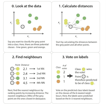
Classification:-
-->Classification is a process of categorizing a given data into different classes.
-->Classification can be performed on both structured or unstructured data to categorize the data.
eg:-Classifying the mail whether it belong spam or not spam


UN SUPERVISED MACHINE LEARNING:-

The linear line is given by the equation


 | = | coefficient of determination |
 | = | sum of squares of residuals |
 | = | total sum of squares |


- R^2 will consider DOB, No of years of Experience & Degree to predict the salary of a person but where as
- Adjusted R^2 will consider No of years of Experience & Degree to predict the salary of a person


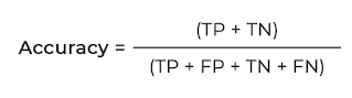
Underfitting is nothing but getting high error with respect to both training dataset & testing dataset. i.e. our model Accuracy will be bad with respect to both training data & testing data
Ridge Regression
- Ridge regression is similar to linear regression, but in ridge regression a small amount of bias is introduced to get the better long-term predictions.
- Ridge Regression will prevent overfitting, so the output of Ridge Regression we get is a generalized model.
- Ridge regression is also called as L2 regularization.
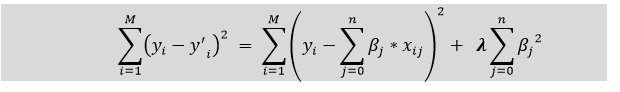
- The penalty which we added to the cost function is called Ridge Regression penalty. Penalty can be calculated by multiplying with the lambda to the squared weight of each individual feature.
- In Ridge regression the co-efficient value(λ) will come near to 'zero' but wont become 'zero'
- Ridge Regression is more preferred for small & medium dimensionality data.
- The equation for the cost function in ridge regression is as follows:
- Lambda(λ) value is selected by using cross-validation.
Lasso Regression:-
- Lasso Regression is also known as L1 Regularization.
- Lasso Regression helps in
2)Perform Feature Selection
- Lasso regression is a type of linear regression but Lasso Regression uses shrinkage.
- Lasso Regression is more preferred when we high dimensions in data
- In Lasso Regression the co-efficient value may become 'zero'
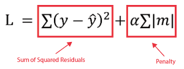
- In above formula we can observe that their was no square to penalty so that the features which are not important are not squared up as of Ridge Regression. So, the value of features which are not important wont increase. In short in Lasso Regression we are reducing the value of cost function by performing the feature selection by not increasing the value of features which are not important
- We Assume that the data follows Normal/Gaussian Distribution
- Scaling(Standardization) of the data is done
- Assuming the data follows Linearity
- Assuming multi-collinearity does not exist. If exist drop one of the highly co-related feature.
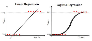
- Logistic Regression algorithm is used for classification problems
- Their are two types of problems statement's in Logistic Regression
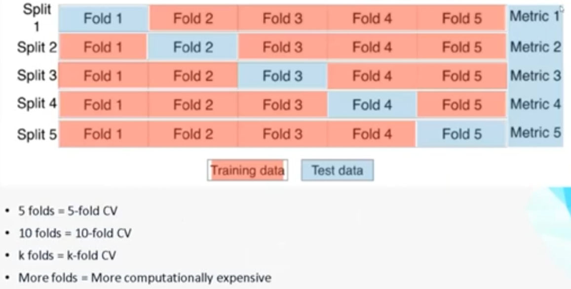
- we use cross validation for not depending on only 1 split, creating multiple splits of data i.e. 5 parts.1part is used for training, remaining for testing, 2nd time 2part is used for training & remaining for testing...…..
- For every round we will calculate error matrix i.e. root mean square error & then mean of all values it is cross validation
- No of folds as we can wish, but we mostly use 5,10 . 10 is most prefered. Size of data is also matters for small data 10folds are not preferred.
- Similarly we have have different ways .They are
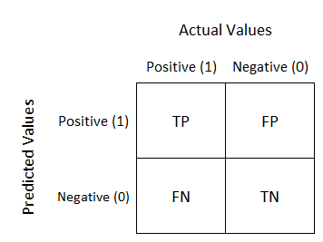
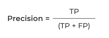
- Whenever FP is more important to reduce use Precision
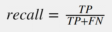
- When ever FN is more important to reduce use Recall
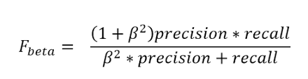
- F0.5-Measure = ((1 + 0.5^2) * Precision * Recall) / (0.5^2 * Precision + Recall)
- F0.5-Measure = (1.25 * Precision * Recall) / (0.25 * Precision + Recall)
- F2-Measure = ((1 + 2^2) * Precision * Recall) / (2^2 * Precision + Recall)
- F2-Measure = (5 * Precision * Recall) / (4 * Precision + Recall)
Working of Naïve Bayes' Classifier:
Lets understood how naive bayes classifier will work by using below example:
Lets take the dataset of weather conditions and corresponding target variable "Play". In the different we have records of different whether conditions and with respect to the corresponding whether condition whether he/she can play or not.
Now by using the dataset we are classifying whether he/she can play when whether is sunny
Solution: To solve this, first consider the below dataset:
Likelihood table weather condition:
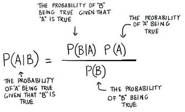
Applying Bayes'theorem:
P(Yes|Sunny)= P(Sunny|Yes)*P(Yes)/P(Sunny)
P(Sunny|Yes)= 3/10= 0.3
P(Sunny)= 0.35
P(Yes)=0.71
So P(Yes|Sunny) = 0.3*0.71/0.35= 0.60
P(No|Sunny)= P(Sunny|No)*P(No)/P(Sunny)
P(Sunny|NO)= 2/4=0.5
P(No)= 0.29
P(Sunny)= 0.35
So P(No|Sunny)= 0.5*0.29/0.35 = 0.41
From above result we can notice that P(Yes|Sunny)>P(No|Sunny)
Hence on a Sunny day, Player can play the game.

- Decision Tree is used to solve both classification & Regression type of Problems.
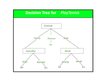
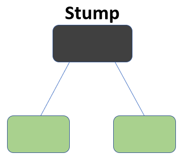
The leaf nodes (green), also called terminal nodes, are nodes that don't split into more nodes.
-->A node is 100% impure when a node is split evenly 50/50 and 100% pure when all of its data belongs to a single class. In order to optimize our model we need to reach maximum purity and avoid impurity.
In decision Tree the purity of the split is measured by
1)Entropy
2)Gini Impurity
The features are selected based on the value of Information Gain
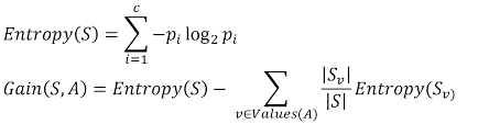
1)Entropy
-->Entropy helps us to build an appropriate decision tree for selecting the best splitter.
-->Entropy can be defined as a measure of the purity of the sub split.
-->Entropy always lies between 0 to 1.
-->The entropy of any split can be calculated by this formula.
Information Gain:-
Information gain is the basic criterion to decide whether a feature should be used to split a node or not. The feature with the optimal split i.e., the highest value of information gain at a node of a decision tree is used as the feature for splitting the node
--->Information Gain is calculated for a split by subtracting the weighted entropies of each branch from the original entropy. When training a Decision Tree using these metrics, the best split is chosen by maximizing Information Gain.
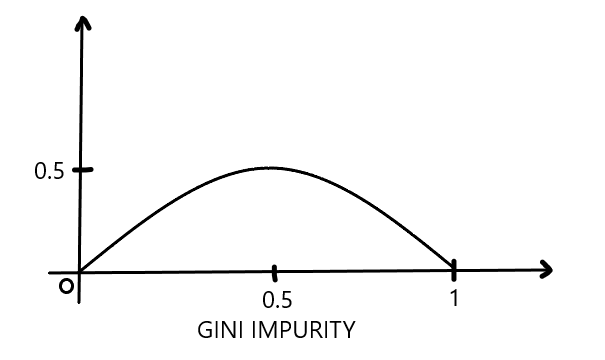
-->Gini impurity has a maximum value of 0.5, which is the worst we can get, and a minimum value of 0 means the best we can get.
Continuous Variable Decision Tree:-
-->A continuous variable decision tree is one where there is not a simple yes or no answer. It’s also known as a regression tree because the decision or outcome variable depends on other decisions farther up the tree or the type of choice involved in the decision.
-->The benefit of a continuous variable decision tree is that the outcome can be predicted based on multiple variables rather than on a single variable as in a categorical variable decision tree
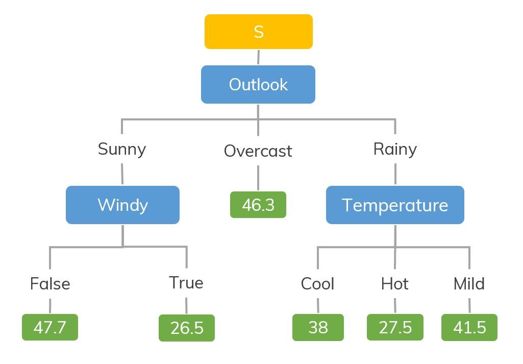
Decision Tree - Regression
Decision tree builds regression or classification models in the form of a tree structure. It breaks down a dataset into smaller and smaller subsets while at the same time an associated decision tree is incrementally developed. The final result is a tree with decision nodes and leaf nodes. A decision node (e.g., Outlook) has two or more branches (e.g., Sunny, Overcast and Rainy), each representing values for the attribute tested. Leaf node (e.g., Hours Played) represents a decision on the numerical target. The topmost decision node in a tree which corresponds to the best predictor called root node. Decision trees can handle both categorical and numerical data.
-->Based on the mean squared error(MSE) the splitting done in regression type of problems in Decision Tree
The strengths of decision tree methods are:
- Decision trees are able to generate understandable rules.
- Decision trees perform classification without requiring much computation.
- Decision trees are able to handle both continuous and categorical variables.
- Decision trees provide a clear indication of which fields are most important for prediction or classification.
The weaknesses of decision tree methods :
- Decision trees are less appropriate for estimation tasks where the goal is to predict the value of a continuous attribute.
- Decision trees are prone to errors in classification problems with many class and relatively small number of training examples.
- Decision tree can be computationally expensive to train. The process of growing a decision tree is computationally expensive. At each node, each candidate splitting field must be sorted before its best split can be found. In some algorithms, combinations of fields are used and a search must be made for optimal combining weights. Pruning algorithms can also be expensive since many candidate sub-trees must be formed and compared.
Hyper parameter tuning:-
Post-Pruning
- This technique is used after construction of decision tree.
- This technique is used when decision tree will have very large depth and will show overfitting of model.
- It is also known as backward pruning.
- This technique is used when we have infinitely grown decision tree.
- Here we will control the branches of decision tree that is
max_depthandmin_samples_splitusingcost_complexity_pruning
- This technique is used before construction of decision tree.
- Pre-Pruning can be done using Hyperparameter tuning.
- Overcome the overfitting issue.
In this blog i will use GridSearchCV for Hyperparameter tuning.
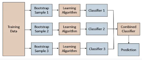
Random Forest is a popular machine learning algorithm that belongs to the supervised learning technique. It can be used for both Classification and Regression problems in ML. It is based on the concept of ensemble learning, which is a process of combining multiple classifiers to solve a complex problem and to improve the performance of the model.
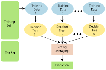
As the name suggests, "Random Forest is a classifier that contains a number of decision trees on various subsets of the given dataset and takes the average to improve the predictive accuracy of that dataset." Instead of relying on one decision tree, the random forest takes the prediction from each tree and based on the majority votes of predictions, and it predicts the final output.
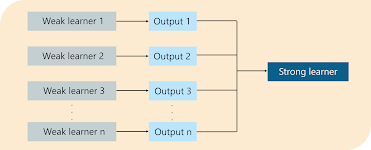
Understanding the working of AdaBoost Algorithm:-
The formula to calculate the sample weights is:
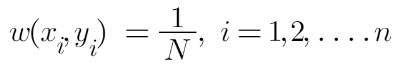
Where N is the total number of datapoints
Step2:-creating a decision stump
We’ll create a decision stump for each of the features and then calculate the Gini Index of each tree. The tree with the lowest Gini Index will be our first stump.
Step3:-Calculating Performance say
We’ll now calculate the “Amount of Say” or “Importance” or “Influence” for this classifier in classifying the datapoints using this formula:
we need to update the weights because if the same weights are applied to the next model, then the output received will be the same as what was received in the first model.
The wrong predictions will be given more weight whereas the correct predictions weights will be decreased. Now when we build our next model after updating the weights, more preference will be given to the points with higher weights.
After finding the importance of the classifier and total error we need to finally update the weights and for this, we use the following formula:
 The amount of say (alpha) will be negative when the sample is correctly classified.
The amount of say (alpha) will be positive when the sample is miss-classified.
Step5:-Creating the buckets
We will create buckets based on Normalized weights
XGBoost:-
-->XGBoost is used for both classification & Regression
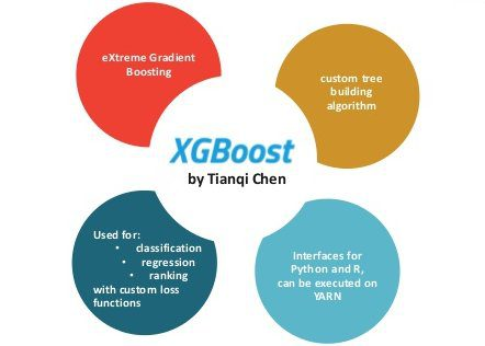


Advantages:-
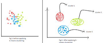
The below are some of the features of K-Means clustering algorithms:
- It is simple to grasp and put into practice.
- K-means would be faster than Hierarchical clustering if we had a high number of variables.
- An instance’s cluster can be changed when centroids are re-computation.
- When compared to Hierarchical clustering, K-means produces tighter clusters.
Disadvantages:-
Some of the drawbacks of K-Means clustering techniques are as follows:
- The number of clusters, i.e., the value of k, is difficult to estimate.
- A major effect on output is exerted by initial inputs such as the number of clusters in a network (value of k).
- The sequence in which the data is entered has a considerable impact on the final output.
- It’s quite sensitive to rescaling. If we rescale our data using normalization or standards, the outcome will be drastically different. ultimate result
- It is not advisable to do clustering tasks if the clusters have a sophisticated geometric shape.
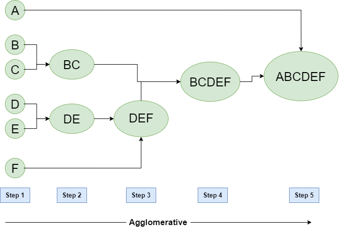
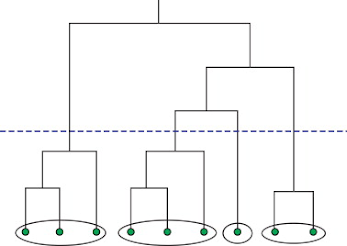
- Step-1:
In Step -1 lets assume each datapoint as a separate cluster and we calculate distance between from one cluster to each and every cluster. - Step-2:
In Step-2 based on the distance between cluster we start grouping clusters. From the above example we can observe that B ,C are nearer to each other . so we form BC as one cluster and D, E are near to each other so we form DE as one cluster - Step-3:
In Step-3 again we calculate the distance between the cluster BC, DE and F and we observed the cluster DE and F are near to each other. So we will form DEF as one cluster. - Step-4:
In Step-4 again we repeat the same above process and BC, DEF are grouped as one cluster as BCDEF - Step-5:
In Step-5 , the two remaining clusters are merged together to form a single cluster as ABCDEF
Silhouette Clustering:-


-->For each data point , we now define

- , if
- -->Silhouette value ranges from -1 to +1, Where a high value indicated that the object is well matched to its own cluster & poorly matched to neighbor cluster similarly vice versa.
- Click here for practical coding part of Silhouette Clustering
DBSCAN Clustering:-
- The full form of DBSCAN is Density-based spatial clustering . DBSCAN is a un-supervised machine learning algorithm used for performing clustering. DBSCAN was proposed by Martin Ester, Hans-Peter Kriegel, Jörg Sander and Xiaowei Xu in 1996.
- -->Take a point & with Eps(Epsilon) distance as a radius, draw a circle, if we give MinPts=4 and no of points lying inside inside circle are minimum 4 then it is called as CORE POINT.
- -->If at least 1 point present inside a circle then it is called as Border Point.
- -->If no point present inside circle then it is called Noise Point.
- -->DBSCAN skips noise points-->Noise point is like a outlier. so we can say that DBSCAN work well with outlier.
- --> -1 cluster is noise point cluster i.e. outliers.


Comments
Post a Comment